Linear Regression에서는 Feature의 수가 많아질 수록 $R^2$가 증가하면서 Overfitting으로 가는 경우가 많다. 그래서 Regularization을 통해서 Overfitting이 되지 않도록 Cost Function 뒤에 Regularization & Labmda(Hyper parameter) Term을 이용해서 조절해준다.
Regularization은 L1-Norm, L2-Norm이 있고, 어떤 것을 쓰는지, 또는 결합하는지에 따라 Ridge, Lasso Regression 또는 Elastic Net으로 분류가 된다.
Norm은 선형대수학에서 유용하게 쓰이는 Operator로 좌표상의 Origin, 즉 원점에서 Vector까지의 거리, Magnitude 를 계산하기 위해 필요하다.
L1 Loss는 LAD(Least Absolute Deviations)라고도 하며 실제값과 예측값 사이의 오차의 절대값을 합한다. 아래 L1 Regularization을 보면 np.linalg.norm을 이용해서 L1 Norm을 취해주었다. - $L=\sum_{i=1}^{n}|y_{i}-f(x_{i})|$
L2 Loss는 LSE(Least Sqaure Error)로 실제값과 예측값 사이의 오차를 제곱하여 합한다. 제곱을 하는 부분 때문에 이상치에 보다 민감한 편이다. - $L=\sum_{i=1}^{n}(y_{i}-f(x_{i}))^{2}$
데이터의 분포가 곡선으로 나올 경우 Feature의 제곱을 추가해줌으로써 비선형모델로 Training을 할 수 있다. 이를 위해서 이용한 함수가 combinations_with_replacement로 feature들을 degree(차수)만큼의 조합으로 생성해낸다.
def normalize(X, axis=-1, order=2):
    """ Normalize the dataset X """
    l2 = np.atleast_1d(np.linalg.norm(X, order, axis))
    l2[l2 == 0] = 1
    return X / np.expand_dims(l2, axis)


def polynomial_features(X, degree):
    n_samples, n_features = np.shape(X)

    def index_combinations():
        combs = [combinations_with_replacement(range(n_features), i) for i in range(0, degree + 1)]
        flat_combs = [item for sublist in combs for item in sublist]
        return flat_combs

    combinations = index_combinations()
    n_output_features = len(combinations)
    X_new = np.empty((n_samples, n_output_features))

    for i, index_combs in enumerate(combinations):
        X_new[:, i] = np.prod(X[:, index_combs], axis=1)

    return X_new

def train_test_split(X, y, test_size=0.5, shuffle=True, seed=None):
    """ Split the data into train and test sets """
    if shuffle:
        X, y = shuffle_data(X, y, seed)
    # Split the training data from test data in the ratio specified in
    # test_size
    split_i = len(y) - int(len(y) // (1 / test_size))
    X_train, X_test = X[:split_i], X[split_i:]
    y_train, y_test = y[:split_i], y[split_i:]

    return X_train, X_test, y_train, y_test


def k_fold_cross_validation_sets(X, y, k, shuffle=True):
    """ Split the data into k sets of training / test data """
    if shuffle:
        X, y = shuffle_data(X, y)

    n_samples = len(y)
    left_overs = {}
    n_left_overs = (n_samples % k)
    if n_left_overs != 0:
        left_overs["X"] = X[-n_left_overs:]
        left_overs["y"] = y[-n_left_overs:]
        X = X[:-n_left_overs]
        y = y[:-n_left_overs]

    X_split = np.split(X, k)
    y_split = np.split(y, k)
    sets = []
    for i in range(k):
        X_test, y_test = X_split[i], y_split[i]
        X_train = np.concatenate(X_split[:i] + X_split[i + 1:], axis=0)
        y_train = np.concatenate(y_split[:i] + y_split[i + 1:], axis=0)
        sets.append([X_train, X_test, y_train, y_test])

    # Add left over samples to last set as training samples
    if n_left_overs != 0:
        np.append(sets[-1][0], left_overs["X"], axis=0)
        np.append(sets[-1][2], left_overs["y"], axis=0)

    return np.array(sets)
Lasso Regression
Lasso는 Least absolute shrinkage and selection operator의 약자이다.
Model의 Bias를 올리면서 Variance Error를 줄이는 방식을 취한다.
Lasso에서 L1-Norm을 사용하면 덜 중요한 변수의 계수를 0으로 수렴하도록 조절할 수 있다. 이 때 적절한 $\lambda$ 설정을 통해서 어느정도까지 변수들을 0으로 수렴하게 할지 결정할 필요가 있다. 이 값은 cross-validation을 통해서 찾게 된다.
Stepwise 대비 일관성있게 변수 선택이 이뤄지는 편이기 때문에 변수 선택 관점에서도 Lasso는 쓸만하다고 볼 수 있다.
class LassoRegression(Regression):
    """Linear regression model with a regularization factor which does both variable selection
    and regularization. Model that tries to balance the fit of the model with respect to the training
    data and the complexity of the model. A large regularization factor with decreases the variance of
    the model and do para.
    Parameters:
    -----------
    degree: int
        The degree of the polynomial that the independent variable X will be transformed to.
    reg_factor: float
        The factor that will determine the amount of regularization and feature
        shrinkage.
    n_iterations: float
        The number of training iterations the algorithm will tune the weights for.
    learning_rate: float
        The step length that will be used when updating the weights.
    """
    def __init__(self, degree, reg_factor, n_iterations=3000, learning_rate=0.01):
        self.degree = degree
        self.regularization = l1_regularization(alpha=reg_factor)
        super(LassoRegression, self).__init__(n_iterations,
                                            learning_rate)

    def fit(self, X, y):
        X = normalize(polynomial_features(X, degree=self.degree))
        super(LassoRegression, self).fit(X, y)

    def predict(self, X):
        X = normalize(polynomial_features(X, degree=self.degree))
        return super(LassoRegression, self).predict(X)
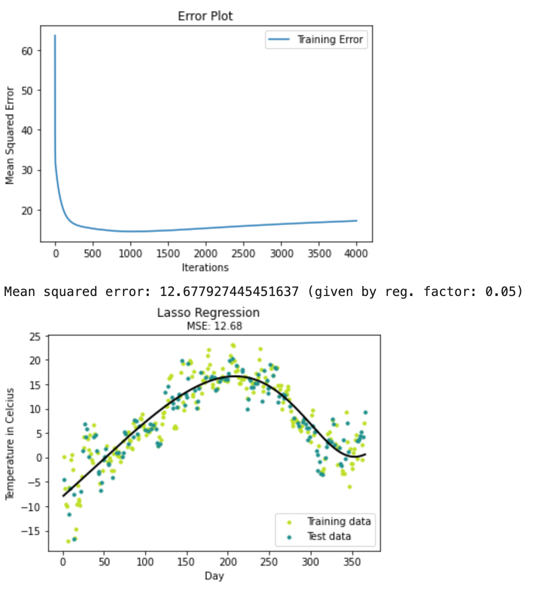
Test & Result
from itertools import combinations_with_replacement
data = pd.read_csv('https://raw.githubusercontent.com/eriklindernoren/ML-From-Scratch/master/mlfromscratch/data/TempLinkoping2016.txt', sep="\t")

time = np.atleast_2d(data["time"].values).T
temp = data["temp"].values

X = time # fraction of the year [0, 1]
y = temp

X_train, X_test, y_train, y_test = train_test_split(X, y, test_size=0.4)

poly_degree = 13

model = LassoRegression(degree=15,
                        reg_factor=0.05,
                        learning_rate=0.001,
                        n_iterations=4000)
model.fit(X_train, y_train)

# Training error plot
n = len(model.training_errors)
training, = plt.plot(range(n), model.training_errors, label="Training Error")
plt.legend(handles=[training])
plt.title("Error Plot")
plt.ylabel('Mean Squared Error')
plt.xlabel('Iterations')
plt.show()

y_pred = model.predict(X_test)
mse = mean_squared_error(y_test, y_pred)
print ("Mean squared error: %s (given by reg. factor: %s)" % (mse, 0.05))

y_pred_line = model.predict(X)

# Color map
cmap = plt.get_cmap('viridis')

# Plot the results
m1 = plt.scatter(366 * X_train, y_train, color=cmap(0.9), s=10)
m2 = plt.scatter(366 * X_test, y_test, color=cmap(0.5), s=10)
plt.plot(366 * X, y_pred_line, color='black', linewidth=2, label="Prediction")
plt.suptitle("Lasso Regression")
plt.title("MSE: %.2f" % mse, fontsize=10)
plt.xlabel('Day')
plt.ylabel('Temperature in Celcius')
plt.legend((m1, m2), ("Training data", "Test data"), loc='lower right')
plt.show()
Ridge Regression
변수 선택보다는 상관성이 있는 변수들에 대해서 적절한 가중치 배분을 하게 된다. 이 부분은 PCA와의 아이디어와도 연결되는 부분이다.
가중치가 Lasso에서는 0이 되지만, Ridge에서는 0이 되지는 않는다. Lasso는 중요한 변수를 선택하는 관점에서 활용할 수 있지만, Ridge는 전체적으로 변수의 중요도가 고만고만하다면 써볼 수 있다.
class PolynomialRegression(Regression):
    """Performs a non-linear transformation of the data before fitting the model
    and doing predictions which allows for doing non-linear regression.
    Parameters:
    -----------
    degree: int
        The degree of the polynomial that the independent variable X will be transformed to.
    n_iterations: float
        The number of training iterations the algorithm will tune the weights for.
    learning_rate: float
        The step length that will be used when updating the weights.
    """
    def __init__(self, degree, n_iterations=3000, learning_rate=0.001):
        self.degree = degree
        # No regularization
        self.regularization = lambda x: 0
        self.regularization.grad = lambda x: 0
        super(PolynomialRegression, self).__init__(n_iterations=n_iterations,
                                                learning_rate=learning_rate)

    def fit(self, X, y):
        X = polynomial_features(X, degree=self.degree)
        super(PolynomialRegression, self).fit(X, y)

    def predict(self, X):
        X = polynomial_features(X, degree=self.degree)
        return super(PolynomialRegression, self).predict(X)

class RidgeRegression(Regression):
    """Also referred to as Tikhonov regularization. Linear regression model with a regularization factor.
    Model that tries to balance the fit of the model with respect to the training data and the complexity
    of the model. A large regularization factor with decreases the variance of the model.
    Parameters:
    -----------
    reg_factor: float
        The factor that will determine the amount of regularization and feature
        shrinkage.
    n_iterations: float
        The number of training iterations the algorithm will tune the weights for.
    learning_rate: float
        The step length that will be used when updating the weights.
    """
    def __init__(self, reg_factor, n_iterations=1000, learning_rate=0.001):
        self.regularization = l2_regularization(alpha=reg_factor)
        super(RidgeRegression, self).__init__(n_iterations,
                                            learning_rate)

class PolynomialRidgeRegression(Regression):
    """Similar to regular ridge regression except that the data is transformed to allow
    for polynomial regression.
    Parameters:
    -----------
    degree: int
        The degree of the polynomial that the independent variable X will be transformed to.
    reg_factor: float
        The factor that will determine the amount of regularization and feature
        shrinkage.
    n_iterations: float
        The number of training iterations the algorithm will tune the weights for.
    learning_rate: float
        The step length that will be used when updating the weights.
    """
    def __init__(self, degree, reg_factor, n_iterations=3000, learning_rate=0.01, gradient_descent=True):
        self.degree = degree
        self.regularization = l2_regularization(alpha=reg_factor)
        super(PolynomialRidgeRegression, self).__init__(n_iterations,
                                                        learning_rate)

    def fit(self, X, y):
        X = normalize(polynomial_features(X, degree=self.degree))
        super(PolynomialRidgeRegression, self).fit(X, y)

    def predict(self, X):
        X = normalize(polynomial_features(X, degree=self.degree))
        return super(PolynomialRidgeRegression, self).predict(X)
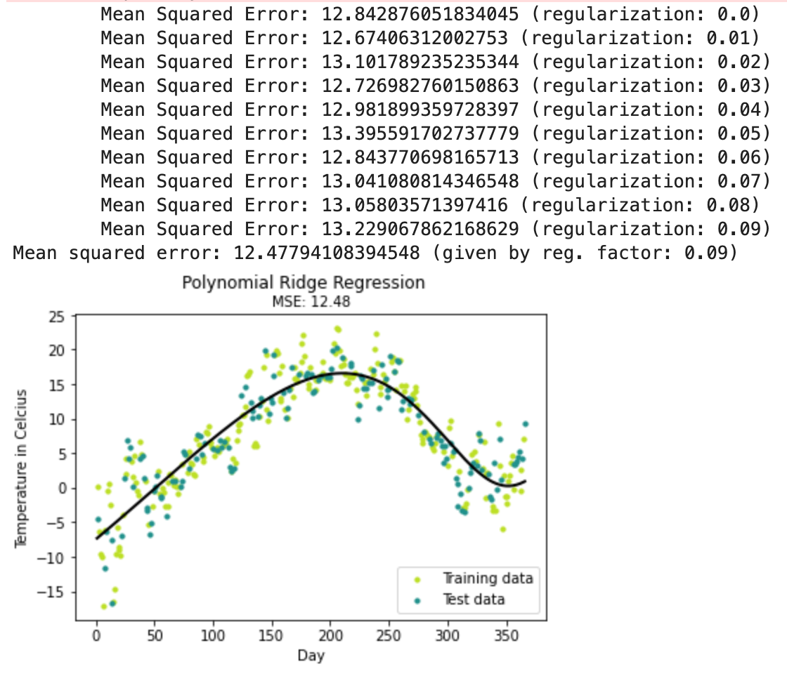
Test & Result
poly_degree = 15

# Finding regularization constant using cross validation
lowest_error = float("inf")
best_reg_factor = None
print ("Finding regularization constant using cross validation:")
k = 10
for reg_factor in np.arange(0, 0.1, 0.01):
    cross_validation_sets = k_fold_cross_validation_sets(
        X_train, y_train, k=k)
    mse = 0
    for _X_train, _X_test, _y_train, _y_test in cross_validation_sets:
        model = PolynomialRidgeRegression(degree=poly_degree,
                                        reg_factor=reg_factor,
                                        learning_rate=0.001,
                                        n_iterations=10000)
        model.fit(_X_train, _y_train)
        y_pred = model.predict(_X_test)
        _mse = mean_squared_error(_y_test, y_pred)
        mse += _mse
    mse /= k

    # Print the mean squared error
    print ("\tMean Squared Error: %s (regularization: %s)" % (mse, reg_factor))

    # Save reg. constant that gave lowest error
    if mse < lowest_error:
        best_reg_factor = reg_factor
        lowest_error = mse

# Make final prediction
model = PolynomialRidgeRegression(degree=poly_degree,
                                reg_factor=reg_factor,
                                learning_rate=0.001,
                                n_iterations=10000)
model.fit(X_train, y_train)

y_pred = model.predict(X_test)
mse = mean_squared_error(y_test, y_pred)
print ("Mean squared error: %s (given by reg. factor: %s)" % (mse, reg_factor))

y_pred_line = model.predict(X)

# Color map
cmap = plt.get_cmap('viridis')

# Plot the results
m1 = plt.scatter(366 * X_train, y_train, color=cmap(0.9), s=10)
m2 = plt.scatter(366 * X_test, y_test, color=cmap(0.5), s=10)
plt.plot(366 * X, y_pred_line, color='black', linewidth=2, label="Prediction")
plt.suptitle("Polynomial Ridge Regression")
plt.title("MSE: %.2f" % mse, fontsize=10)
plt.xlabel('Day')
plt.ylabel('Temperature in Celcius')
plt.legend((m1, m2), ("Training data", "Test data"), loc='lower right')
plt.show()
Elastic Net
Elastic Net은 Lasso와 Ridge를 절충한 모델
Lasso는 아래 제약조건의 영역(파란색 부분)이 마름모, Ridge는 원으로 형성되고 저 안에 들어오는 값이 Feasible Set으로 최적값이 되는데, 지금 아래 그림을 보면 알 수 있듯이 마름모도 아니고 원도 아닌, 중간 형태를 취하고 있는 것을 볼 수 있다.
Lasso는 다중공선성이 높으면 성능이 좋지 않고, Ridge는 변수 선택기능이 없는데, 이 두부분을 Elastic Net은 Cover할 수 있다.
그래서 아래 모델을 보면 l1_l2_regularization(alpha=reg_factor, l1_ratio=l1_ratio)이라는 부분이 Elastic Net의 핵심부분이다.
class ElasticNet(Regression):
    """ Regression where a combination of l1 and l2 regularization are used. The
    ratio of their contributions are set with the 'l1_ratio' parameter.
    Parameters:
    -----------
    degree: int
        The degree of the polynomial that the independent variable X will be transformed to.
    reg_factor: float
        The factor that will determine the amount of regularization and feature
        shrinkage.
    l1_ration: float
        Weighs the contribution of l1 and l2 regularization.
    n_iterations: float
        The number of training iterations the algorithm will tune the weights for.
    learning_rate: float
        The step length that will be used when updating the weights.
    """
    def __init__(self, degree=1, reg_factor=0.05, l1_ratio=0.5, n_iterations=3000,
                learning_rate=0.01):
        self.degree = degree
        self.regularization = l1_l2_regularization(alpha=reg_factor, l1_ratio=l1_ratio)
        super(ElasticNet, self).__init__(n_iterations,
                                        learning_rate)

    def fit(self, X, y):
        X = normalize(polynomial_features(X, degree=self.degree))
        super(ElasticNet, self).fit(X, y)

    def predict(self, X):
        X = normalize(polynomial_features(X, degree=self.degree))
        return super(ElasticNet, self).predict(X)


Member discussion